Learning Objectives

• Practice optimisation and how algorithms can reduce computation time
• Apply optimisation techniques to root finding.

Optimisation

Optimisation is another important skill which underlies many data analysis techniques. This area is vast so will use a relatively easy example to show how algorithms can significantly reduce the computation time.

Today we will focus on finding roots using two different algorithms: bisection and Newton-Raphson.

Bisection

The below graph shows the equation $y = x^2 \sin(x) - e^x$.

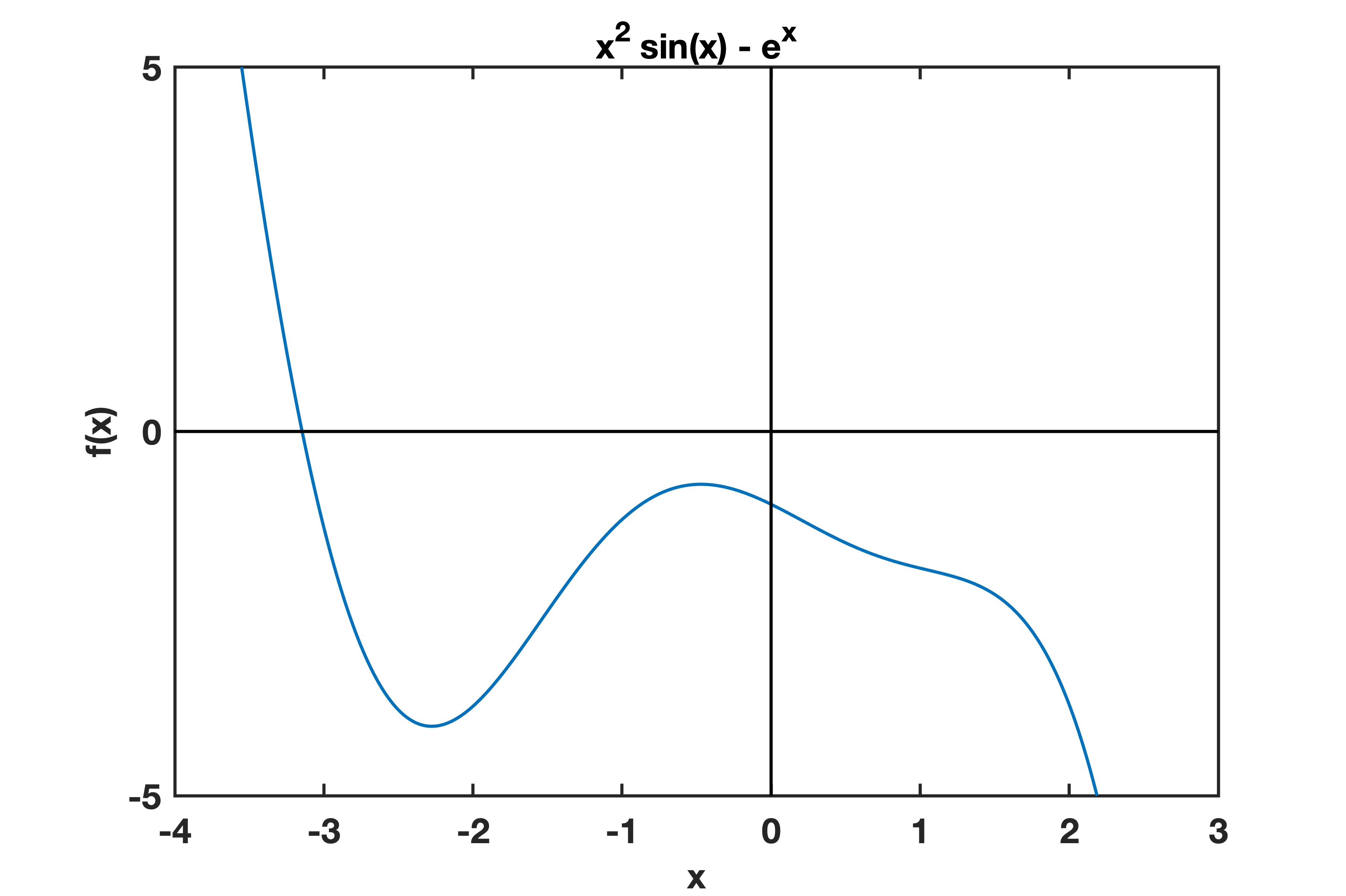
One method of finding the root of an equation is bisection. When there is a root, there typically is a change of sign (positive to negative). Looking at our example equation from above, we can see that the function has a root about x = −3. A bisection algorithm takes two points, x0 and x2, and finds the midpoint, x1. If there is a change of sign when we evaluate these values, there is a root within these boundaries. below is one implementation of the bisection method:

function [root,error,iterations] = find_root(initial_x,fun)
error = 1;
tolerance = 0.01;
x = initial_x;
delta_x = 1.0001;
iterations = 0;
while error > tolerance && iterations < 10000
    iterations = iterations+1;
    y0 = fun(x);
    y1 = fun(x+delta_x);
    y2 = fun(x+2*delta_x);

    if y0/y1 < 0
        delta_x = delta_x/2;
        error = abs(delta_x/(x+delta_x));
    elseif y2/y1 < 0
        delta_x = delta_x/2;
        error = abs(delta_x/(x+delta_x));
        x = x+delta_x;
    else 
        x = x+2*delta_x;
    end
end

root = x;
end

Task 9a

Using the line coefficients from the projectile question (8b), create a function which takes an input time and outputs the displacement.

Task 9b

Use the bisection method from above to find roots. Try different values of intitial_x and tolerance and see how this affects the answer.

Newton-Rapson

This is the most widely used of all root-locating formulas. One way of deriving the Newton-Rhapson formula is by graphical derivation:

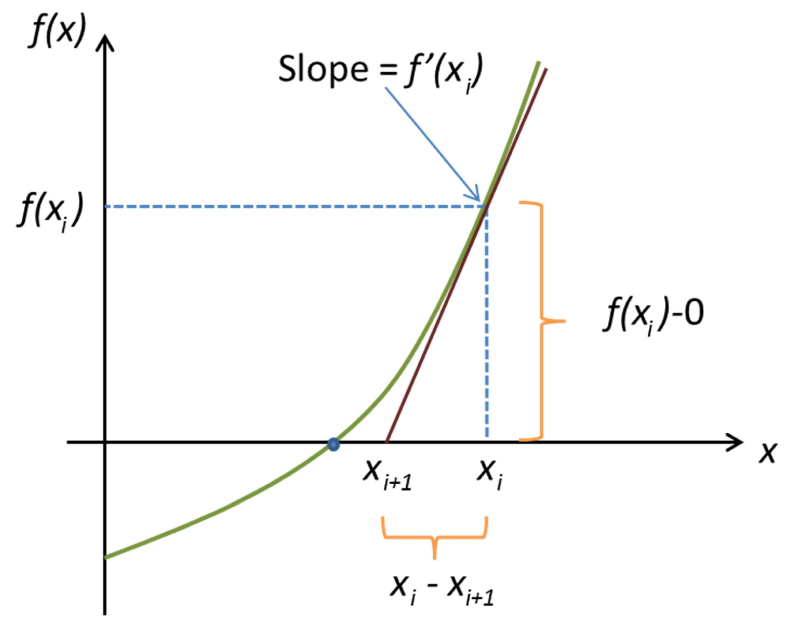
The Newton-Rapson method is given as: $x_{i+1} = x_i - \frac{f(x_i)}{f’(x_i)}$

where $f’(x)$ is the derivative or gradient of function $f(x)$, $x_{i+1}$ is the next best guess for the root, and $x$ is the current guess for the root. This process can repeat many times to find a root to greater accuracy. normally we only care about a certain degree of accuracy!

This equation assumes we know the gradient of the function. If this is not known, then we can approximate by taking a small step, ∆, in either direction and calculating the gradient (for example ∆ = 0.001): $f’(x_i) = \frac{f(x+\Delta) -f(x-\Delta)}{2 \Delta}$

Below is a working implementation of the Newton-Rapson method.

function [root,error,iterations] = NewtonRaphson(initial_x,fun)

error = 1;
tolerance = 0.00001;
x = initial_x;
delta_x = 0.001;
iterations = 0;

while error > tolerance && iterations <100
    iterations = iterations + 1;
    est_grad = (fun(x+delta_x)-fun(x-delta_x))/(2*delta_x);
    x_new = x - fun(x)/est_grad;
    error = abs(x-x_new);
    x = x_new;
end

root = x;
end

Task 9c

Try the Newton-Rapson method with the same function. Compare how quickly the roots are found by the number of iterations compared to the bisection method.

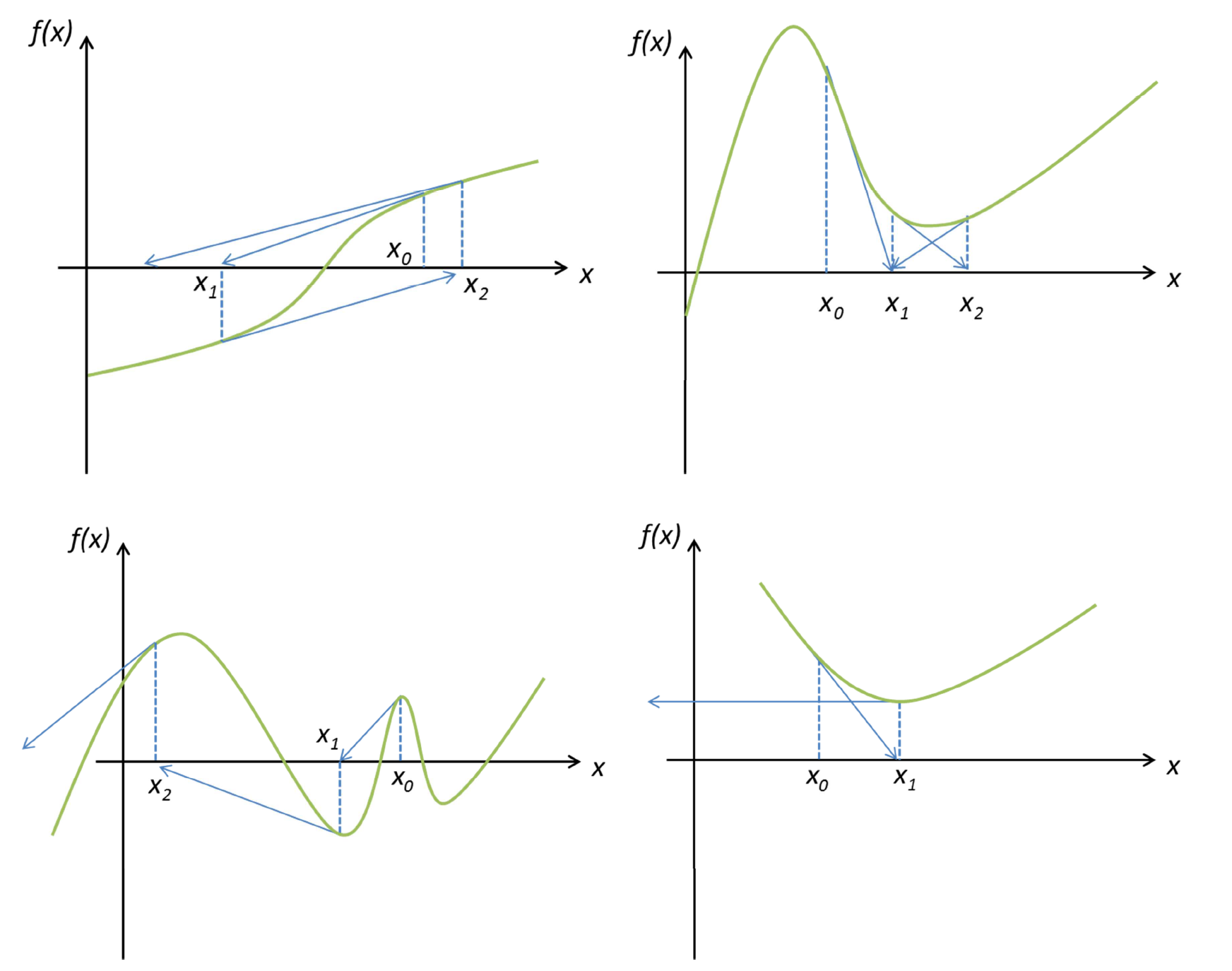
When Newton-Rapson breaks down

Sometimes algorithms break down. Below shows some cases when Newton-Rapson breaks down.

Task 9d

How might you address bad initial guesses, and how can we sure of how many roots there are?

Bonus

Try your idea with the following function:

function y = fun1(x)
y = (x+1).*(x-2).*(x+2);
end